Smooth propensity
Model startup
Any strategy pattern you implement should take into account the fact that in the early days of the model its predictions are likely to be erratic. As the model matures, its predictive power improves. To facilitate usage of the model in the beginning, we have introduced the concept of Smooth Propensity.
Formula
A propensity smoothing mechanism is used to jump start the process. Propensity smoothing requires an assumed starting propensity and an assumed amount of starting evidence. The evidence is the number of proposition responses that contributed to the propensity for a particular proposition. When no response data has been received, the smoothed propensity equals the starting propensity. The recommended formula for propensity smoothing, as defined in the expression editor, is:
(@divide(.StartingEvidence, (.StartingEvidence + .ModelEvidence+1.0),3) * .StartingPropensity) +
(@divide(.ModelEvidence, (.StartingEvidence + .ModelEvidence+1.0), 3)*.pyPropensity)
Where:
Starting Evidence and Starting Propensity are proposition properties representing the assumed values for evidence and propensity.
Model Evidence and Model Performance are the actual outputs of the adaptive model (set on the Output mappings tab), pyPropensity is the main model output.
Convergence
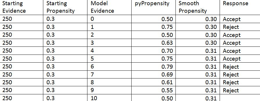
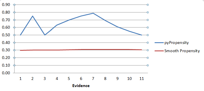
The example table and graph below show how volatile model propensity can be following the initial responses to an offer.
As responses are recorded, the starting propensity value converges with the actual propensity. Let’s consider a scenario in which the starting evidence and starting propensity are 50 and 0.30 respectively.
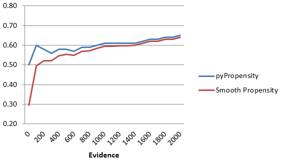
When there are as many responses as starting evidence, the starting and actual propensities are equally important. When the number of actual responses becomes much higher than the starting evidence, the smoothed propensity converges with the actual propensity. The graph above exhibits this pattern.